Starting with data
Data Carpentry contributors
Learning Objectives
- Load external tabular data from a .csv file into R.
- Describe what an R data frame is.
- Summarize the contents of a data frame in R.
- Manipulate categorical data in R using factors.
Looking at Metadata
We are studying a population of Escherichia coli (designated Ara-3), which were propagated for more than 40,000 generations in a glucose-limited minimal medium. This medium was supplemented with citrate which E. coli cannot metabolize in the aerobic conditions of the experiment. Sequencing of the populations at regular time points reveals that spontaneous citrate-using mutants (Cit+) appeared at around 31,000 generations. This metadata describes information on the Ara-3 clones and the columns represent:
| Column | Description |
|---|---|
| sample | clone name |
| generation | generation when sample frozen |
| clade | based on parsimony-based tree |
| strain | ancestral strain |
| cit | citrate-using mutant status |
| run | Sequence read archive sample ID |
| genome_size | size in Mbp (made up data for this lesson) |
The metadata file required for this lesson can be downloaded directly here or viewed in Github.
Tip: If you can’t find the Ecoli_metadata.csv file, or have lost track of it, download the file directly using the R
download.file() function
download.file("https://raw.githubusercontent.com/datacarpentry/R-genomics/gh-pages/data/Ecoli_metadata.csv", "data/Ecoli_metadata.csv")You are now ready to load the data. We are going to use the R function read.csv() to load the data file into memory (as a data.frame):
metadata <- read.csv('data/Ecoli_metadata.csv')This statement doesn’t produce any output because assignment doesn’t display anything. If we want to check that our data has been loaded, we can print the variable’s value: metadata
Alternatively, wrapping an assignment in parentheses will perform the assignment and display it at the same time.
(metadata <- read.csv('data/Ecoli_metadata.csv'))## sample generation clade strain cit run genome_size
## 1 REL606 0 <NA> REL606 unknown 4.62
## 2 REL1166A 2000 unknown REL606 unknown SRR098028 4.63
## 3 ZDB409 5000 unknown REL606 unknown SRR098281 4.60
## 4 ZDB429 10000 UC REL606 unknown SRR098282 4.59
## 5 ZDB446 15000 UC REL606 unknown SRR098283 4.66
## 6 ZDB458 20000 (C1,C2) REL606 unknown SRR098284 4.63
## 7 ZDB464* 20000 (C1,C2) REL606 unknown SRR098285 4.62
## 8 ZDB467 20000 (C1,C2) REL606 unknown SRR098286 4.61
## 9 ZDB477 25000 C1 REL606 unknown SRR098287 4.65
## 10 ZDB483 25000 C3 REL606 unknown SRR098288 4.59
## 11 ZDB16 30000 C1 REL606 unknown SRR098031 4.61
## 12 ZDB357 30000 C2 REL606 unknown SRR098280 4.62
## 13 ZDB199* 31500 C1 REL606 minus SRR098044 4.62
## 14 ZDB200 31500 C2 REL606 minus SRR098279 4.63
## 15 ZDB564 31500 Cit+ REL606 plus SRR098289 4.74
## 16 ZDB30* 32000 C3 REL606 minus SRR098032 4.61
## 17 ZDB172 32000 Cit+ REL606 plus SRR098042 4.77
## 18 ZDB158 32500 C2 REL606 minus SRR098041 4.63
## 19 ZDB143 32500 Cit+ REL606 plus SRR098040 4.79
## 20 CZB199 33000 C1 REL606 minus SRR098027 4.59
## 21 CZB152 33000 Cit+ REL606 plus SRR097977 4.80
## 22 CZB154 33000 Cit+ REL606 plus SRR098026 4.76
## 23 ZDB83 34000 Cit+ REL606 minus SRR098034 4.60
## 24 ZDB87 34000 C2 REL606 plus SRR098035 4.75
## 25 ZDB96 36000 Cit+ REL606 plus SRR098036 4.74
## 26 ZDB99 36000 C1 REL606 minus SRR098037 4.61
## 27 ZDB107 38000 Cit+ REL606 plus SRR098038 4.79
## 28 ZDB111 38000 C2 REL606 minus SRR098039 4.62
## 29 REL10979 40000 Cit+ REL606 plus SRR098029 4.78
## 30 REL10988 40000 C2 REL606 minus SRR098030 4.62Wow… that was a lot of output. At least it means the data loaded properly. Let’s check the top (the first 6 lines) of this data.frame using the function head():
head(metadata)## sample generation clade strain cit run genome_size
## 1 REL606 0 <NA> REL606 unknown 4.62
## 2 REL1166A 2000 unknown REL606 unknown SRR098028 4.63
## 3 ZDB409 5000 unknown REL606 unknown SRR098281 4.60
## 4 ZDB429 10000 UC REL606 unknown SRR098282 4.59
## 5 ZDB446 15000 UC REL606 unknown SRR098283 4.66
## 6 ZDB458 20000 (C1,C2) REL606 unknown SRR098284 4.63Note
read.csvassumes that fields are delineated by commas, however, in several countries, the comma is used as a decimal separator and the semicolon (;) is used as a field delineator. If you want to read in this type of files in R, you can use theread.csv2function. It behaves exactly likeread.csvbut uses different parameters for the decimal and the field separators. If you are working with another format, they can be both specified by the user. Check out the help forread.csv()to learn more.
We’ve just done two very useful things. 1. We’ve read our data in to R, so now we can work with it in R 2. We’ve created a data frame (with the read.csv command) the standard way R works with data.
What are data frames?
data.frame is the de facto data structure for most tabular data and what we use for statistics and plotting.
A data.frame is a collection of vectors of identical lengths. Each vector represents a column, and each vector can be of a different data type (e.g., characters, integers, factors). The str() function is useful to inspect the data types of the columns.
A data.frame can be created by the functions read.csv() or read.table(), in other words, when importing spreadsheets from your hard drive (or the web).
By default, data.frame converts (= coerces) columns that contain characters (i.e., text) into the factor data type. Depending on what you want to do with the data, you may want to keep these columns as character. To do so, read.csv() and read.table() have an argument called stringsAsFactors which can be set to FALSE:
Let’s now check the __str__ucture of this data.frame in more details with the function str():
str(metadata)## 'data.frame': 30 obs. of 7 variables:
## $ sample : Factor w/ 30 levels "CZB152","CZB154",..: 7 6 18 19 20 21 22 23 24 25 ...
## $ generation : int 0 2000 5000 10000 15000 20000 20000 20000 25000 25000 ...
## $ clade : Factor w/ 7 levels "(C1,C2)","C1",..: NA 7 7 6 6 1 1 1 2 4 ...
## $ strain : Factor w/ 1 level "REL606": 1 1 1 1 1 1 1 1 1 1 ...
## $ cit : Factor w/ 3 levels "minus","plus",..: 3 3 3 3 3 3 3 3 3 3 ...
## $ run : Factor w/ 30 levels "","SRR097977",..: 1 5 22 23 24 25 26 27 28 29 ...
## $ genome_size: num 4.62 4.63 4.6 4.59 4.66 4.63 4.62 4.61 4.65 4.59 ...Inspecting data.frame objects
We already saw how the functions head() and str() can be useful to check the content and the structure of a data.frame. Here is a non-exhaustive list of functions to get a sense of the content/structure of the data.
- Size:
dim()- returns a vector with the number of rows in the first element, and the number of columns as the second element (the __dim__ensions of the object)nrow()- returns the number of rowsncol()- returns the number of columns
- Content:
head()- shows the first 6 rowstail()- shows the last 6 rows
- Names:
names()- returns the column names (synonym ofcolnames()fordata.frameobjects)rownames()- returns the row names
- Summary:
str()- structure of the object and information about the class, length and content of each columnsummary()- summary statistics for each column
Note: most of these functions are “generic”, they can be used on other types of objects besides data.frame.
Challenge
Based on the output of
str(metadata), can you answer the following questions?
- What is the class of the object
metadata?- How many rows and how many columns are in this object?
- How many citrate+ mutants have been recorded in this population?
As you can see, many of the columns in our data frame are of a special class called factor. Before we learn more about the data.frame class, we are going to talk about factors. They are very useful but not necessarily intuitive, and therefore require some attention.
Factors
When we did str(metadata) we saw that several of the columns consist of integers, however, the columns clade, strain, cit, run, … are of a special class called a factor. Factors are very useful and are actually something that make R particularly well suited to working with data, so we’re going to spend a little time introducing them.
Factors are used to represent categorical data. Factors can be ordered or unordered and are an important class for statistical analysis and for plotting.
Factors are stored as integers, and have labels associated with these unique integers. While factors look (and often behave) like character vectors, they are actually integers under the hood, and you need to be careful when treating them like strings.
In the data frame we just imported, let’s do
str(metadata)## 'data.frame': 30 obs. of 7 variables:
## $ sample : Factor w/ 30 levels "CZB152","CZB154",..: 7 6 18 19 20 21 22 23 24 25 ...
## $ generation : int 0 2000 5000 10000 15000 20000 20000 20000 25000 25000 ...
## $ clade : Factor w/ 7 levels "(C1,C2)","C1",..: NA 7 7 6 6 1 1 1 2 4 ...
## $ strain : Factor w/ 1 level "REL606": 1 1 1 1 1 1 1 1 1 1 ...
## $ cit : Factor w/ 3 levels "minus","plus",..: 3 3 3 3 3 3 3 3 3 3 ...
## $ run : Factor w/ 30 levels "","SRR097977",..: 1 5 22 23 24 25 26 27 28 29 ...
## $ genome_size: num 4.62 4.63 4.6 4.59 4.66 4.63 4.62 4.61 4.65 4.59 ...We can see the names of the multiple columns. And, we see that some say things like Factor w/ 3 levels
You can learn what these level are by using the function levels(),
levels(metadata$cit)## [1] "minus" "plus" "unknown"and check the number of levels using nlevels():
nlevels(metadata$cit)## [1] 3When we read in a file, any column that contains text is automatically assumed to be a factor. Once created, factors can only contain a pre-defined set values, known as levels. By default, R always sorts levels in alphabetical order.
For instance, we see that cit is a Factor w/ 3 levels, minus, plus and unknown.
Sometimes, the order of the factors does not matter, other times you might want to specify the order because it is meaningful (e.g., “low”, “medium”, “high”), it improves your visualization, or it is required by a particular type of analysis. Here, one way to reorder our levels in the cit vector would be:
cit <-metadata$cit
cit # current order
## [1] unknown unknown unknown unknown unknown unknown unknown unknown
## [9] unknown unknown unknown unknown minus minus plus minus
## [17] plus minus plus minus plus plus minus plus
## [25] plus minus plus minus plus minus
## Levels: minus plus unknowncit <- factor(cit, levels = c("plus", "minus", "unknown"))
cit # after re-ordering## [1] unknown unknown unknown unknown unknown unknown unknown unknown
## [9] unknown unknown unknown unknown minus minus plus minus
## [17] plus minus plus minus plus plus minus plus
## [25] plus minus plus minus plus minus
## Levels: plus minus unknownChallenge
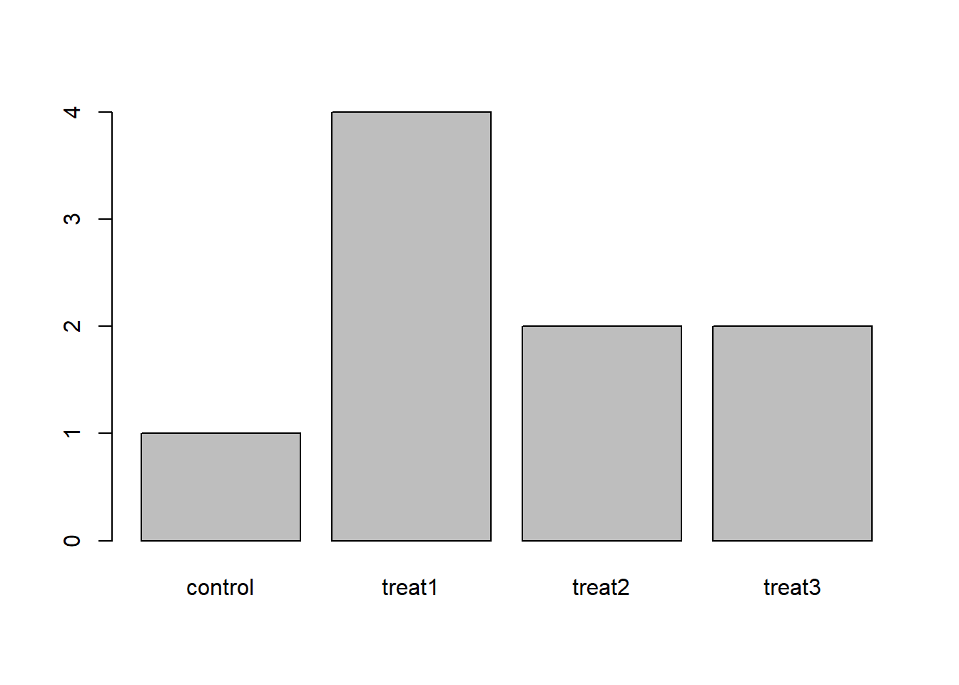
The function
table()tabulates observations and can be used to create bar plots quickly. For instance:
- Question: How can you recreate this plot but by having “control” being listed last instead of first?
exprmt <- factor(c("treat1", "treat2", "treat1", "treat3", "treat1", "control",
                  "treat1", "treat2", "treat3"))
table(exprmt)
## exprmt ## control treat1 treat2 treat3 ## 1 4 2 2barplot(table(exprmt))
In R’s memory, these factors are represented by integers (1, 2, 3), but are more informative than integers because factors that are self describing: "plus", "minus" is more descriptive than 1, 2. Which one is “plus”? You wouldn’t be able to tell just from the integer data. Factors, on the other hand, have this information built in. It is particularly helpful when there are many levels (like the strains in our example dataset).
Converting factors
If you need to convert a factor to a character vector, you use as.character(x).
as.character(cit)## [1] "unknown" "unknown" "unknown" "unknown" "unknown" "unknown" "unknown"
## [8] "unknown" "unknown" "unknown" "unknown" "unknown" "minus" "minus"
## [15] "plus" "minus" "plus" "minus" "plus" "minus" "plus"
## [22] "plus" "minus" "plus" "plus" "minus" "plus" "minus"
## [29] "plus" "minus"Converting factors where the levels appear as numbers (such as concentration levels, generations or years) to a numeric vector is a little trickier.
Lets simulate an error in importing the dataset where generation was misidentified as a factor rather than a integer
generation <- factor(metadata$generation) The as.numeric() function returns the index values of the factor, not its levels, so it will result in an entirely new (and unwanted in this case) set of numbers. One method to avoid this is to convert factors to characters and then numbers.
Another method is to use the levels() function. Compare:
as.numeric(generation) # Wrong! And there is no warning...## [1] 1 2 3 4 5 6 6 6 7 7 8 8 9 9 9 10 10 11 11 12 12 12 13
## [24] 13 14 14 15 15 16 16as.numeric(as.character(generation)) # Works...## [1] 0 2000 5000 10000 15000 20000 20000 20000 25000 25000 30000
## [12] 30000 31500 31500 31500 32000 32000 32500 32500 33000 33000 33000
## [23] 34000 34000 36000 36000 38000 38000 40000 40000as.numeric(levels(generation))[generation] # The recommended way.## [1] 0 2000 5000 10000 15000 20000 20000 20000 25000 25000 30000
## [12] 30000 31500 31500 31500 32000 32000 32500 32500 33000 33000 33000
## [23] 34000 34000 36000 36000 38000 38000 40000 40000Notice that in the levels() approach, three important steps occur:
- We obtain all the factor levels using
levels(generation) - We convert these levels to numeric values using
as.numeric(levels(generation)) - We then access these numeric values using the underlying integers of the vector
generationinside the square brackets
The automatic conversion of data type is sometimes a blessing, sometimes an annoyance. Be aware that it exists, learn the rules, and double check that data you import in R are of the correct type within your data frame. If not, use it to your advantage to detect mistakes that might have been introduced during data entry (a letter in a column that should only contain numbers for instance).
Renaming factors
When your data is stored as a factor, you can use the plot() function to get a quick glance at the number of observations represented by each factor level. Let’s look at the number of citrate-using mutants (Cit+) over the course of the experiment:
## bar plot of the number of clade in the samples:
plot(metadata$cit)
In addition to minus and plus, there are about 12 samples for which the cit information hasn’t been recorded. Additionally, for these individuals, there is no label to indicate that the information is missing. Let’s rename this label to something more meaningful. Before doing that, we’re going to pull out the data on cit mutant status and work with that data, so we’re not modifying the working copy of the data frame
cit <- metadata$cit
head(cit)
## [1] unknown unknown unknown unknown unknown unknown
## Levels: minus plus unknownlevels(cit)## [1] "minus" "plus" "unknown"head(cit)## [1] unknown unknown unknown unknown unknown unknown
## Levels: minus plus unknownChallenge
- Rename “minus” and “plus” to “negative” and “postive” respectively.
Data Carpentry,
2017. License. Contributing.
Questions? Feedback?
Please file
an issue on GitHub.
On
Twitter: @datacarpentry